While conventional social network analysis is highly exploratory and descriptive in nature, there is an increasing need for scalable computational tools enabling robust prediction and decision making for dynamic networks. Several aspects of this problem make it fundamentally challenging. First, the number of observations may be very small relative to the size of the social network; this “data-starved” setting makes devising statistically robust and computationally efficient methods especially difficult. Second, the observations are typically incomplete, in that many attributes are not recorded, and noisy or erroneous. Third, social networks of interest are very large, necessitating scalable tool development. Fourth, in many real-world settings we do not have access to all events at once, which precludes batch processing and necessitates online methods instead. Finally, the mechanism underlying the observed events may be dynamically changing. To overcome these challenges, there is a need for novel theory and methods that exploit low-dimensional structure in the dynamic geometry of social networks. This is a dramatic shift from previous work in social network analysis. In particular, the low-dimensional topological structure of social networks shapes the pattern of information diffusion, and the latter shapes the dynamics of the former. Understanding these interactions is a crucial component of robust and efficient dynamic social network prediction and decision theory.

Co-occurrence data can represent critical information in a variety of contexts, such as meetings in a social network, routers in a communication network, or genes, proteins, and metabolites in biological networks. In particular, a single co-occurrence observation indicates a subset of entities (people, routers, genes, etc.) which all participate in an event; understanding the underlying co-occurrence patterns for a series of events makes it possible to identify correlations among the entities beyond simple pair-wise analyses. Furthermore, accurately predicting future co-occurrences based on previous observations can aid in filtering, changepoint estimation, and anomaly detection. However, these tasks are complicated by several challenges: (a) the networks considered may be very large, (b) the subset of entities participating in a single event may also be large, (c) sequential observations may have hidden dependencies or even be contaminated by an adversary, and (d) it is critical to detect changing patterns with as few observations as possible. We have developed an online convex programming approach to sequential probability assignment of high-dimensional co-occurrence data.

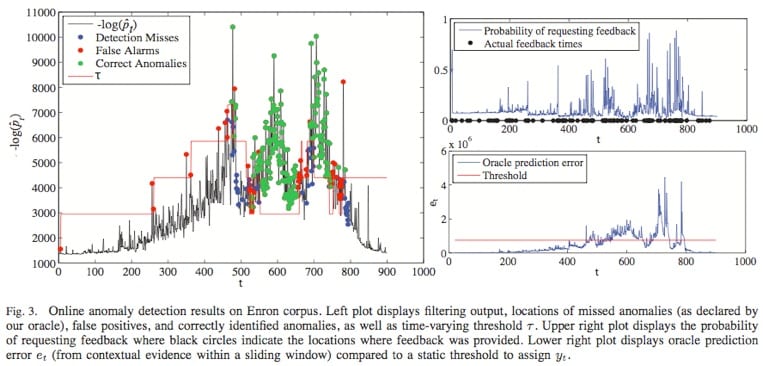
Our approach consists of two main elements: (1) filtering, or assigning a belief or likelihood to each successive measurement based upon our ability to predict it from previous noisy observations, and (2) hedging, or flagging potential anomalies by comparing the current belief against a time-varying and data-adaptive threshold. The threshold is adjusted based on the available feedback from an end user. Our algorithms, which combine universal prediction with recent work on online convex programming, do not require computing posterior distributions given all current observations and involve simple primal-dual parameter updates. At the heart of the proposed approach lie exponential-family models which can be used in a wide variety of contexts and applications, and which yield methods that achieve sublinear per-round regret against both static and slowly varying product distributions with marginals drawn from the same exponential family. Moreover, the regret against static distributions coincides with the minimax value of the corresponding online strongly convex game. We also prove bounds on the number of mistakes made during the hedging step relative to the best offline choice of the threshold with access to all estimated beliefs and feedback signals. We validate the theory on synthetic data drawn from a time-varying distribution over binary vectors of high dimensionality, as well as on the Enron email dataset.

Sequential detection of anomalous communication patterns

For example, when monitoring interactions within a social network, meetings or contacts between different members of the network are recorded: these meetings constitute observations of a point process. NISLab lab has addressed the problem of using the recorded meetings to determine (a) whether each meeting is anomalous and (b) the degree to which each meeting is anomalous. Performing robust statistical analysis on such data is particularly challenging when the number of observed meetings is much smaller than the number of people in the network. Our novel approach to anomaly detection in this high-dimensional setting is based on hypergraphs, an important extension of graphs which allows edges to connect more than two vertices simultaneously. This is a significant paradigm change from conventional approaches, which model the social network as a graph, weighing graph edges by the number of observed meetings, and using standard graph-theoretic algorithms to conduct inference. Such approaches have several disadvantages, including high computational complexities and an inherent loss of critical information due to the nature of the data structures employed.

Furthermore, we have applied our method to a real, large scale social network: the Enron email database (see www.cs.cmu.edu/~enron), which contains approximately half a million emails involving over 75,000 addresses.

 

Batch anomaly detection in static social networks

NISLab has also developed a novel framework based upon a variational Expectation-Maximization algorithm to assess the likelihood of each observation being anomalous. The computational complexity of the proposed method scales linearly with both the number of observed events and the number of people in the network, while most competing methods exhibit far worse complexities which scale quadratically with the number of people in the network or the number of meetings observed. This makes our method much more well-suited to very large networks, and it requires no parameter tuning. In our simulations, we were able to detect anomalous meetings within a 2000-person network with 100% accuracy using just 200 observations, while alternative approaches based on graphs were significantly more computationally expensive and alternative approaches based on Support Vector Machines resulted in large numbers of falsely detected anomalous meetings.

 

Code

You need the following file: demo_varem (just the variational EM). Inside, you’ll find two .mat files with the preprocessed Enron dataset. You’ll also find three scripts: “demo_synthetic.m”, “demo_enron_subject.m” and “demo_enron_day.m”, which exemplify how to call all the other functions. Run either of these, for results with synthetic data or the Enron data, organized by subject line or by day, respectively.

Additionally, you should download and install the lightspeed toolbox for MATLAB from Tom Minka’s page, because of the “logsumexp” function and other improvements: lightspeed toolbox.

With the synthetic example, you can set the parameters by editing “demo_synthetic.m”. You shouldn’t decrease the number of observations much lower than n=200, unless the dimensionality p is low. You can crank up p as far as your memory will allow. In a laptop with 2 GB RAM, if you keep the MC sample size down at m=1000 and set, say, n=200, you should be able to go as far as p=20,000. The Enron example, organized by day, has p=75,511.

 

Comparison with other methods

If you intend to run the comparison with the OCSVM algorithm, you’ll need to use the file: demo_ocsvm.zip (Variational EM vs. OCSVM) and also download and install the libsvm toolbox for MATLAB, by Chih-Chung Chang and Chih-Jen Lin: libsvm toolbox. Tip: to get libsvm working on some platforms, you may need to edit “make.m” and replace all references to .obj with .o instead.

For comparing with L1O-kNNG, we have included a (probably rather crude) implementation: l1o_knng(Variational EM vs. L1O-kNNG).

Extract all the demo_*.zip files to the same directory. Remember to add the toolbox locations to your MATLAB path. Then, run “demo_ocsvm.m” or “demo_l1o_knng.m”. Optionally, you can also just edit “demo_synthetic.m” to set parameters and to mix and match methods for comparison (simply set the corresponding run_* variables equal to one, in the “Initialization” section of the code) and then run the edited “demo_synthetic.m”.